Hello there, I have had a look at a rather similar thread (link here) but despite a lot of tinkering about I cannot get it to function to my requirements.
Currently I am using the following formula:
=INDEX('Finance Billing Periods'!A:F,MATCH('Period List'!D6,'Finance Billing Periods'!B:B,),1,1)
in the "Billing Period" column on TABLE 1, which pulls from the data in TABLE 2
TABLE 1
(Columns A, B & C)
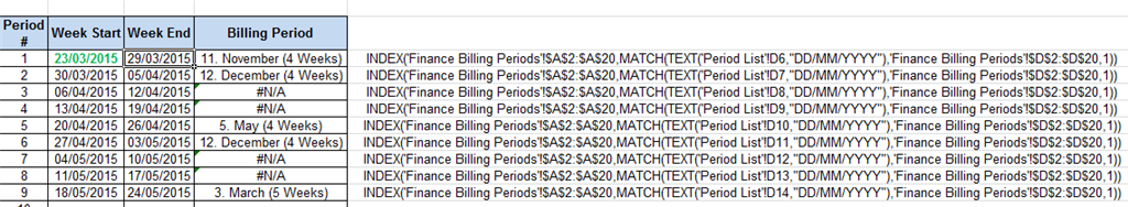
| Week Start | Week End | Billing Period |
| 23/03/2015 | 29/03/2015 | 4. April (4 Weeks) |
| 30/03/2015 | 05/04/2015 | - |
| 06/04/2015 | 12/04/2015 | - |
| 13/04/2015 | 19/04/2015 | - |
| 20/04/2015 | 26/04/2015 | 5. May (4 Weeks) |
| 27/04/2015 | 03/05/2015 | - |
| 04/05/2015 | 10/05/2015 | - |
| 11/05/2015 | 17/05/2015 | - |
| 18/05/2015 | 24/05/2015 | 6. June (4 Weeks) |
TABLE 2
(Columns A,B,C,D,E,F & G)
| Billing Period | Start Time | End Time | Start Date Only | End Date Only | Duration | Weeks |
| A | 17/05/2014 00:00 | 20/06/2014 23:59 | 17/05/2014 | 20/06/2014 | 34.99930556 | 5 |
| B | 21/06/2014 00:00 | 18/07/2014 17:00 | 21/06/2014 | 18/07/2014 | 27.70833333 | 4 |
| C | 19/07/2014 00:00 | 15/08/2014 17:00 | 19/07/2014 | 15/08/2014 | 27.70833333 | 4 |
| D | 16/08/2014 00:00 | 19/09/2014 17:00 | 16/08/2014 | 19/09/2014 | 34.70833333 | 5 |
| E | 20/09/2014 00:00 | 17/10/2014 17:00 | 20/09/2014 | 17/10/2014 | 27.70833333 | 4 |
| F | 18/10/2014 00:00 | 14/11/2014 17:00 | 18/10/2014 | 14/11/2014 | 27.70833333 | 4 |
| G | 15/11/2014 00:00 | 12/12/2014 17:00 | 15/11/2014 | 12/12/2014 | 27.70833333 | 4 |
| 1. January (5 Weeks) | 15/12/2014 00:00 | 16/01/2015 23:59 | 15/12/2014 | 16/01/2015 | 32.99930556 | 5 |
| 2. February (4 Weeks) | 19/01/2015 00:00 | 13/02/2015 23:59 | 19/01/2015 | 13/02/2015 | 25.99930556 | 4 |
| 3. March (5 Weeks) | 16/02/2015 00:00 | 20/03/2015 23:59 | 16/02/2015 | 20/03/2015 | 32.99930556 | 5 |
| 4. April (4 Weeks) | 23/03/2015 00:00 | 17/04/2015 23:59 | 23/03/2015 | 17/04/2015 | 25.99930556 | 4 |
| 5. May (4 Weeks) | 20/04/2015 00:00 | 15/05/2015 23:59 | 20/04/2015 | 15/05/2015 | 25.99930556 | 4 |
| 6. June (4 Weeks) | 18/05/2015 00:00 | 19/06/2015 23:59 | 18/05/2015 | 19/06/2015 | 32.99930556 | 5 |
| 7. July (4 Weeks) | 22/06/2015 00:00 | 17/07/2015 23:59 | 22/06/2015 | 17/07/2015 | 25.99930556 | 4 |
| 8. August (4 Weeks) | 20/07/2015 00:00 | 14/08/2015 23:59 | 20/07/2015 | 14/08/2015 | 25.99930556 | 4 |
| 9. September (5 Weeks) | 17/08/2015 00:00 | 18/09/2015 23:59 | 17/08/2015 | 18/09/2015 | 32.99930556 | 5 |
| 10. October (4 Weeks) | 21/09/2015 00:00 | 16/10/2015 23:59 | 21/09/2015 | 16/10/2015 | 25.99930556 | 4 |
| 11. November (4 Weeks) | 19/10/2015 00:00 | 20/11/2015 23:59 | 19/10/2015 | 20/11/2015 | 32.99930556 | 5 |
| 12. December (4 Weeks) | 23/11/2015 00:00 | 18/12/2015 23:59 | 23/11/2015 | 18/12/2015 | 25.99930556 | 4 |
I am trying to get enter a formula that says if the two dates in TABLE 1 are in the range from TABLE 2 (Start Date Only and End Date Only) then pull out the Billing Period from TABLE 2.
IE: like below in TABLE 3:
TABLE 3
(Columns A, B & C)
| Week Start | Week End | Billing Period |
| 23/03/2015 | 29/03/2015 | 4. April (4 Weeks) |
| 30/03/2015 | 05/04/2015 | 4. April (4 Weeks) |
| 06/04/2015 | 12/04/2015 | 4. April (4 Weeks) |
| 13/04/2015 | 19/04/2015 | 4. April (4 Weeks) |
| 20/04/2015 | 26/04/2015 | 5. May (4 Weeks) |
| 27/04/2015 | 03/05/2015 | 5. May (4 Weeks) |
| 04/05/2015 | 10/05/2015 | 5. May (4 Weeks) |
| 11/05/2015 | 17/05/2015 | 5. May (4 Weeks) |
| 18/05/2015 | 24/05/2015 | 6. June (4 Weeks) |
Is this something that is possible to achieve? I have messed about with the formula from the post I mentioned at the top and came up with this formula which is just returning blanks so it's probably wrong, or I'm wrong somewhere!
=IFERROR(INDEX('Finance Billing Periods'!D1:E20,SMALL(IF(FREQUENCY(IF('Finance Billing Periods'!D1:D20>='Period List'!D6,IF('Finance Billing Periods'!E1:E20<='Period List'!E6,MATCH(D6:D83,D6:D83,0))),ROW('Finance Billing Periods'!D2:D20)-ROW('Finance Billing Periods'!D$2)),ROW('Finance Billing Periods'!D2:D20)-ROW('Finance Billing Periods'!D2)),COUNTA(G$5:G5))),"")
Appreciate in advance any suggestions & assistance. I don't mind what type of formula is required to achieve this so feel free to suggest any alternative. :)


 This sheet is called "Period List". I'm not mistyping as I'm just selecting the range from within the formula.