
Hello
Please could you help me write a formula to calculate a 5 year long service award on an annual leave sheet.
Here is what I have at the moment

At the moment its not doing exactly what I want.
The formula working out 60 months is in F5 and is =DATEDIF(E5,A9,"m") - E5 is the start date A9 is todays date.
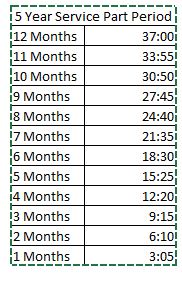
the formula working out 37:00 hours is =IF(F5>59,"37:00","") - it should say 15:25 - here's why.
If this staff member reaches 5 years service part way through the period, they are not entitled to five full days, they are only entitled to 5 months of that long service award which is 15 hours and 25 minutes. (They accrue 3 hours and 05 minutes per month)
The way I Imagine its done is if we have a formula working out how many months it is from their 5 year anniversary, until the following 31/03/####, and then alter =IF(F5>59,"37:00","") to display the correct number of hours and minutes dependent on that figure? Or is there a better way of doing it?
(Of course the next 31/03/#### would need to be variable as staff join at different years)
Once they reach the next 1st April, they are then entitled to the 5 full days so the formula would need to stop counting at that point leaving them with 37:00
Hope this makes sense?
Here is the monthly accruement chart
Many thanks
Luke


