Formula Help with Building a Mileage log and fuel use spreadsheet

Hello,

I have a fleet of 17 trucks that I need to monitor mileage on and the spreadsheet that was built for us by an outside source never did function correctly.

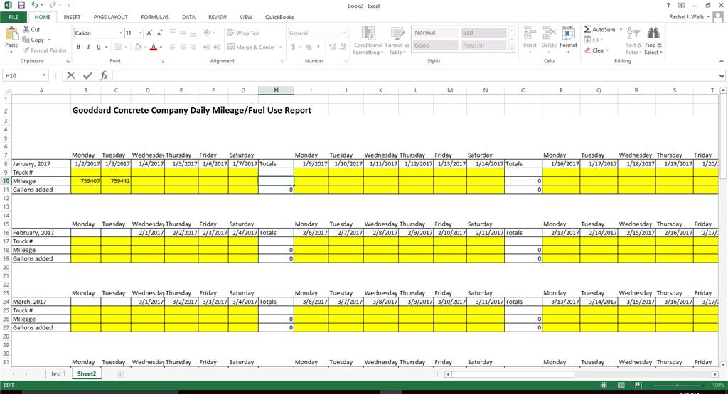
I have the structure built the way I would like it to look and run. I just need a formula that will figure it correctly. I need it to total the mileage weekly, monthly and yearly. I can handle the month and yearly totals but I cannot get it to figure the miles traveled correctly.

I have a row for mileage (Row 10). I have it divided into weekly blocks (Mon - Sat) inside the month spread with a totals needed at the end of the week block.

Which begins at Row 10 and needs to total columns B thru G as miles traveled totals shown in Row 10 Column H.

I have attached a screenshot of the spreadsheet with the first two mileage entered in the correct cells and the total in the "totals cell" should be 34.

If I can just get some help with this first block of total miles I can adjust the formula for the rest of the spreadsheet.

Not all trucks are run everyday so I will need to factor in there might not be a number in a column for one or two days. 

Then at the end of the month I am needing to add all of those weekly totals together. I'm pretty sure I won't have a problem getting the monthly total since I will just have to add only certain cells for a total.

Any help would be greatly appreciated!!

Hi Rachel,

Unfortunately, you're going to drive yourself absolutely nuts trying to track with that format.

You'll be better off thinking transactionally, where each truck/day has its own row. That way you can easily summarize over any time period with PivotTables.

Something like this:

The nice thing about using PivotTables is that as you add new data, you simply refresh them to instantly see the new data summarized. And you can easily group by Week/Month, etc.

Every once in a while there's a sudden gust of gravity...

Was this reply helpful?

Sorry this didn't help.

Great! Thanks for your feedback.

How satisfied are you with this reply?

Thanks for your feedback, it helps us improve the site.

How satisfied are you with this reply?

Thanks for your feedback.

SmittyPro's advice is worth heeding.

If you want to stick with what you've got, a formula in H10 to get the mileage can be:

=MAX(B10:G10)-MIN(B10:G10)

Regards

Murray
https://excel.dadsonion.com

Was this reply helpful?

Sorry this didn't help.

Great! Thanks for your feedback.

How satisfied are you with this reply?

Thanks for your feedback, it helps us improve the site.

How satisfied are you with this reply?

Thanks for your feedback.

Thanks for the info. I would definitely like to build a table like that eventually. I am reteaching myself as I go, I don't have a lot of experience with excel and what I did learn was 10+ years ago lol and if you don't use it you lose it. I will look into that. Thank you.

Was this reply helpful?

Sorry this didn't help.

Great! Thanks for your feedback.

How satisfied are you with this reply?

Thanks for your feedback, it helps us improve the site.

How satisfied are you with this reply?

Thanks for your feedback.

Thank you for this formula! It has worked perfectly. I will look into building the PivotTables, I just needed something that would function now.

Was this reply helpful?

Sorry this didn't help.

Great! Thanks for your feedback.

How satisfied are you with this reply?

Thanks for your feedback, it helps us improve the site.

How satisfied are you with this reply?

Thanks for your feedback.

{snip} I will look into building the PivotTables {snip}

Here's a tutorial: Create a PivotTable to analyze data.

Every once in a while there's a sudden gust of gravity...

Was this reply helpful?

Sorry this didn't help.

Great! Thanks for your feedback.

How satisfied are you with this reply?

Thanks for your feedback, it helps us improve the site.

How satisfied are you with this reply?

Thanks for your feedback.


Question Info


Last updated October 5, 2021 Views 485 Applies to: