Office 365 Mac - Excel - Pivot Table Issue

I have never created a Pivot table and despite trying to set up one, I am not smart enough to figure out. (Never needed to create a Pivot table.) People that work with such day to day, it would be like falling off log to create one).

------------------

However I have found a Mistake in your math. To get the right sum you:

• Format Cells B2 through H4 as Numbers with one decimal place. (0.0 - 1.0)
• The if you go to Formulas
• First click in cell F5
• Then Click AutoSum. 
• Total will be 1.5

As you can see  total is 1.5 not 1.4

Even the row the AutoSum totals are in, have to be formatted number, with 1 decimal point. If two decimal points are used you may get the 1.4 total.  Also your entries in the pivot table are suspect. Looks like subtracted -.1, from each number how did that happen. 

_________

Disclaimer:

The questions, discussions, opinions, replies & answers I create, are solely mine and mine alone, and do not reflect upon my position as a Community Moderator.

You are certainly entitled to your opinions about Mac Excel, but there are millions of users who think otherwise and use it every day.

in the case at hand, you need to take a good look at the source data details. Quite likely there is significant data to the right of the tenths position. Are you sure it is the same on both platforms? How did you make the screen shots? Did you open the exact same file in both platforms, or did you move the data from one platform to the other and then create the pivot table? Are you sure the pivot source was refreshed before making the screen shots?

Bob,

I recreated on Preview his chart using his Figures. And With the Exception Of my using The "Classic" look which use Grey main Section and Green Status Bar, instead of the Opposite. He did use Mac Preview Version. 

I used his own numbers. However The Format for the cells with the numbers, including the Row below the last numbers I set to:

Numbers

1 Decimal Place

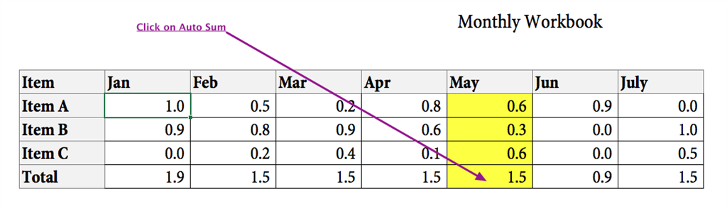
When I click on Formulas:

I clicked in Cell below all the numbers in the May Column and clicked on AutoSum

As you can See the total I came up with was 1.5. 

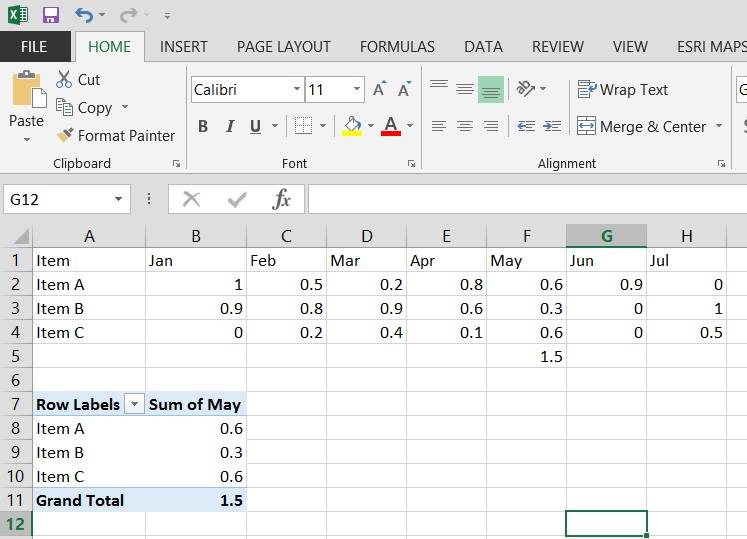
I don't know anything about Pivot tables to comment on them although it appears the .1 was subtracted from results of each item.

What shows in his Pivot table instead of .6, .3, .6 which when either

added  =F2 + F3 + F4 or

AutoSum= F2:F4

Both come out as 1.5

Something doesn't seem right.  If I could Just figure out How to do a Pivot Table I could double check his Pivot table Figures.

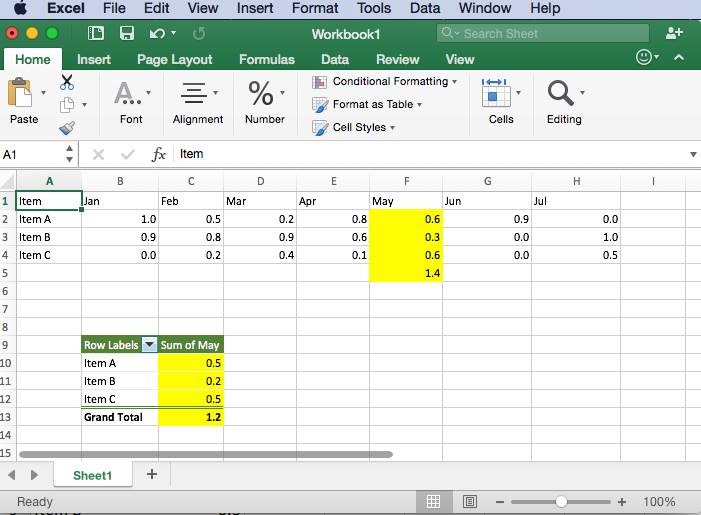
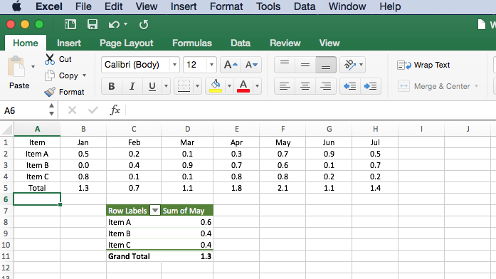
Okay I just Tried again. And although not like his I sort of created a simple Pivot table:

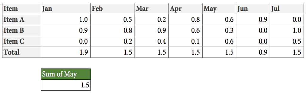
 I went to Insert Menu, then Pivot Table and went into Pivot table Builder. I selected  May, and then for rows I selected F2:F4 which ended up with this when finished.

I feel like that. he didn't format the Data correctly. 

_________

Disclaimer:

The questions, discussions, opinions, replies & answers I create, are solely mine and mine alone, and do not reflect upon my position as a Community Moderator.

If you were to share the files you took screen shots of we can tell you how the data is different between the two pivottables. To share the files, upload them to a file sharing service such as OneDrive.com or DropBox.com (both services are free). Then reply with links to the files.

Excel on the Mac has no known calculation deficiencies in this regard in all versions, including the Preview edition.

Hi Jim (& Phillip):

As background, the numbers were generated using the RAND() function, then rounded down to the decimal point you see in the graphic.  I can somewhat understand that the decimal addition could be off due to rounding, however the Auto SUM() function was used thereafter in the original file.  

After updating Preview yesterday, I was able to reproduce the Pivot Table issue once again, however it appears that Auto SUM() function has been fixed as I wasn't able to reproduce that issue again; possibly fixed by latest update?  Don't know.

However, as you can see, in generating a new pivot table on the selected data, the Pivot Table is throwing in numbers that do not correlate correctly to the May column.

The link to the below graphic/workbook is here: http://1drv.ms/1GqKpeI

I have no need to duplicate the file for MS-Office 365 in Windows as it is not the issue/concern here.

Thanks, Don

Thanks Bob; glad you value my opinion.  

There was significant data to the right of the tenths position and subsequently rounded down.  The data from MS-Excel Preview was copied and pasted exactly as shown into MS-Excel for Office 365 for Windows and generated the end result. Auto Sum was used to add the columns for both instances.  How did I make the screenshots?  How does that factor in?  Really?

Pivot source was refreshed for both instances prior to any screenshots capture and the data did not change in either instance. Pivot table was imbedded into same workbook as the data/table.

Please see the follow-up in the latest entry below and research the attached workbook in that entry as you see fit.  

Screenshots?  Again, really?

Sorry I am Going to have to Bow out. I can't even Get Pivot table to work for me. At all either in 2011 nor 2016 will Not let me pick out individual Row and Column headers and Sums the count of the cells.

Have JE or one of the other help.

_________
Disclaimer:
The questions, discussions, opinions, replies & answers I create, are solely mine and mine alone, and do not reflect upon my position as a Community Moderator.

Well, I sure don't see the issue.

Send a screen shot with one of the data cells selected. You said the data was created by RAND and then rounded. Was it rounded by formatting? If so, the original data to 15 digits of significance is still in the cell.

Bob,

Here is a fresh screenshot for you and the workbook was posted as requested, earlier in this thread. Does May (Pivot Table) match May's data? I don't think so. A picture (and workbook) are a thousand words.

Bob, 

Okay the I think I figured out Even Though I can't Figure out how to set up a Pivot Table It's because he is using the Ran() (Random) function which generates a Random number each and every time The Chart/Range/ Spreadsheet is refreshed or updated.

Bob G has been using mine based on my Chart Which entered numbers not Random.

The Pivot table will always work right with constant numbers. And always fail with Random numbers because even numbers in the pivot table are randomly generated and has nothing to do with numbers in actual Chart the Pivot table is based on. 

Am I on right track?

_________

Disclaimer:

The questions, discussions, opinions, replies & answers I create, are solely mine and mine alone, and do not reflect upon my position as a Community Moderator.